#coin flip model with random 1/survived 0/died

#iterate over dataFrame rows as (index, Series) pairs: https://pandas.pydata.org/pandas-docs/stable/generated/pandas.DataFrame.iterrows.html
for index, row in data1.iterrows():
    #random number generator: https://docs.python.org/2/library/random.html
    if random.random() > .5:     # Random float x, 0.0 <= x < 1.0
        data1.set_value(index, 'Random_Predict', 1) #predict survived/1
    else:
        data1.set_value(index, 'Random_Predict', 0) #predict died/0


# coin flip 모델의 성능을 검증해보자. 옳게 맞추면 1, 아니면 0이다.
#the mean of the column will then equal the accuracy
data1['Random_Score'] = 0 #assume prediction wrong 초기화
data1.loc[(data1['Survived'] == data1['Random_Predict']), 'Random_Score'] = 1 #set to 1 for correct prediction
print('Coin Flip Model Accuracy: {:.2f}%'.format(data1['Random_Score'].mean()*100)) # 평균치를 구한다.

# 혹은 그냥 내장 함수를 사용하자.
#http://scikit-learn.org/stable/modules/generated/sklearn.metrics.accuracy_score.html#sklearn.metrics.accuracy_score
print('Coin Flip Model Accuracy w/SciKit: {:.2f}%'.format(metrics.accuracy_score(data1['Survived'], data1['Random_Predict'])*100))

#group by or pivot table: https://pandas.pydata.org/pandas-docs/stable/generated/pandas.DataFrame.groupby.html
pivot_female = data1[data1.Sex=='female'].groupby(['Sex','Pclass', 'Embarked','FareBin'])['Survived'].mean()
print('Survival Decision Tree w/Female Node: \n',pivot_female)

pivot_male = data1[data1.Sex=='male'].groupby(['Sex','Title'])['Survived'].mean()
print('\n\nSurvival Decision Tree w/Male Node: \n',pivot_male)

#handmade data model using brain power (and Microsoft Excel Pivot Tables for quick calculations)
def mytree(df):

    #initialize table to store predictions
    Model = pd.DataFrame(data = {'Predict':[]})
    male_title = ['Master'] #survived titles

    for index, row in df.iterrows():

        #Question 1: Were you on the Titanic; majority died 타이타닉에 있으면 일단 죽었다고 가정
        Model.loc[index, 'Predict'] = 0

        #Question 2: Are you female; majority survived : 여자는 살았다고 가정
        if (df.loc[index, 'Sex'] == 'female'):
                  Model.loc[index, 'Predict'] = 1

        #Question 3A Female - Class and Question 4 Embarked gain minimum information
        #클래스에 따라 나누는 것은 큰 정보이득이 없다. (즉, 클래스에 따른 생존률의 차이가 없다. 정보이득이 없다. 고르게 분포되어 있어 분기를 만드는 것이 의미가 없다.)

        #Question 5B Female - FareBin; set anything less than .5 in female node decision tree back to 0
        # 여자이며 클래스가 3번, 출항 항구가 S 그리고 돈을 8보다 많이 낸 사람들은 생존했다. 아마 못사는 사람들이 돈을 더 많이 내지 않았을까..
        if ((df.loc[index, 'Sex'] == 'female') &
            (df.loc[index, 'Pclass'] == 3) &
            (df.loc[index, 'Embarked'] == 'S')  &
            (df.loc[index, 'Fare'] > 8)

           ):
                  Model.loc[index, 'Predict'] = 0

        #Question 3B Male: Title; set anything greater than .5 to 1 for majority survived
        # master 지위를 가진 사람만 생존했다고 가정하자.그럼 남자중 57%는 생존했다고 할 수 있다.
        if ((df.loc[index, 'Sex'] == 'male') &
            (df.loc[index, 'Title'] in male_title)
            ):
            Model.loc[index, 'Predict'] = 1

    return Model


#model data
Tree_Predict = mytree(data1)
print('Decision Tree Model Accuracy/Precision Score: {:.2f}%\n'.format(metrics.accuracy_score(data1['Survived'], Tree_Predict)*100))


#Accuracy Summary Report with http://scikit-learn.org/stable/modules/generated/sklearn.metrics.classification_report.html#sklearn.metrics.classification_report
#Where recall score = (true positives)/(true positive + false negative) w/1 being best:http://scikit-learn.org/stable/modules/generated/sklearn.metrics.recall_score.html#sklearn.metrics.recall_score
#And F1 score = weighted average of precision and recall w/1 being best: http://scikit-learn.org/stable/modules/generated/sklearn.metrics.f1_score.html#sklearn.metrics.f1_score
print(metrics.classification_report(data1['Survived'], Tree_Predict))

#Plot Accuracy Summary
#Credit: http://scikit-learn.org/stable/auto_examples/model_selection/plot_confusion_matrix.html
import itertools
def plot_confusion_matrix(cm, classes,
                          normalize=False,
                          title='Confusion matrix',
                          cmap=plt.cm.Blues):
    """
    This function prints and plots the confusion matrix.
    Normalization can be applied by setting `normalize=True`.
    """
    if normalize:
        cm = cm.astype('float') / cm.sum(axis=1)[:, np.newaxis] # 차원을 하나 늘려 세로로 만들어주는 개념
        print("Normalized confusion matrix")
    else:
        print('Confusion matrix, without normalization')

    print(cm)

    plt.imshow(cm, interpolation='nearest', cmap=cmap)
    plt.title(title)
    plt.colorbar()
    tick_marks = np.arange(len(classes))
    plt.xticks(tick_marks, classes, rotation=45)
    plt.yticks(tick_marks, classes)

    fmt = '.2f' if normalize else 'd'
    thresh = cm.max() / 2.
    for i, j in itertools.product(range(cm.shape[0]), range(cm.shape[1])):
        plt.text(j, i, format(cm[i, j], fmt),
                 horizontalalignment="center",
                 color="white" if cm[i, j] > thresh else "black")

    plt.tight_layout()
    plt.ylabel('True label')
    plt.xlabel('Predicted label')

# Compute confusion matrix
cnf_matrix = metrics.confusion_matrix(data1['Survived'], Tree_Predict)
np.set_printoptions(precision=2)

class_names = ['Dead', 'Survived']
# Plot non-normalized confusion matrix
plt.figure()
plot_confusion_matrix(cnf_matrix, classes=class_names,
                      title='Confusion matrix, without normalization')

# Plot normalized confusion matrix
plt.figure()
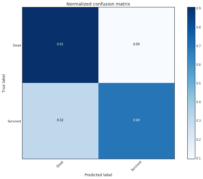
plot_confusion_matrix(cnf_matrix, classes=class_names, normalize=True,
                      title='Normalized confusion matrix')